MEV Tax Distribution

Angstrom L2 captures priority-fee MEV inside the Uniswap v4 hook and pays it out immediately. This note explains how the hook splits the tax between fee recipients and how liquidity providers receive their share. The first section summarizes the on-chain flow; the remainder reproduces the full compensation-price derivation used by the contracts.

How the Tax Flows to LPs

1. Snapshot state: beforeSwap stores the pre-swap tick and liquidity so the hook knows exactly which ranges were crossed.
2. Compute base deltas: TickIteratorLib walks the crossed ticks to derive each range's token deltas.
3. Solve for a uniform price: CompensationPriceFinder chooses a compensation price p* so makers are paid as if the entire swap cleared at that level, using the formulas derived below.
4. Accrue rewards: PoolRewardsLib updates growth accumulators (rewardGrowthOutsideX128, globalGrowthX128) that mirror Uniswap v3/v4 fee accounting.
5. Pay on exit: When LPs remove liquidity, afterRemoveLiquidity settles their accumulated native-token rewards. Integrators can also query getPendingPositionRewards mid-position.

The hook shares the tax between the pool creator, protocol treasury, and LPs according to the fee configuration stored in the factory. LP payouts always stay in the rollup's native asset, matching the currency that sequencers prioritize.

Detailed Compensation Price Derivation

This section ports the formal derivation from the contracts repository. It defines the compensation price $p_\star$ that equalizes maker payoffs when a swap crosses multiple ticks.

Variables & Definitions

• $L_i > 0$: virtual liquidity for range $i$ ($L_i = \sqrt{x_i y_i}$ where $x_i, y_i$ are the virtual reserves for range $i$)
• $p_{i} > 0$ is the price of the lower boundary of range $i$
• $p_\star > 0$: post-trade effective compensation price
• $B > 0$ is the bid/liquidity compensation amount.
• Given some liquidity $L_i$ and a price $p$ we can determine the virtual reserves in $x$ & $y$ at that price point with: $x = L_i\cdot\frac{1}{\sqrt p}, y = L_i\cdot{\sqrt p}$
• To compute the net amount deltas required to cross a range $i$: $\Delta x_i =L_i(\frac{1}{\sqrt{p_i}}-\frac{1}{\sqrt{p_{i+1}}}),\ \Delta y_i = L_i(\sqrt{p_{i+1}}-\sqrt{p_i})$
• $\hat X, \hat Y > 0$: aggregated swap amount of whole ranges where the final $p_\star \notin [a_i, b_i]$ is known to lie outside of (where $a_i = \max\{p_i, p_{\text{start}}\}, b_i = \min\{p_{i+1}, p_{\text{end}}\}$, implicitly $a_i \le b_i$):

$\hat X =\sum_i L_i(\frac{1}{\sqrt{a_i}}-\frac{1}{\sqrt{b_i}}),\qquad \hat Y = \sum_i L_i(\sqrt{b_i}-\sqrt{a_i}).$

Compensation Price definition

Assuming unsigned total deltas $X = \sum_i {\Delta x_i}, Y=\sum_i \Delta y_i$ the final compensation price $p_\star$ is defined as:

Zero-for-One Swap: $p_\star = \frac{Y}{X + B}$ such that each range $i$ trades $\Delta x_i' = \Delta y_i \cdot (\min\{p_\star, \frac{\Delta y_i}{\Delta x_i}\})^{-1}$

One-for-Zero Swap: $p_\star = \frac{Y}{X- B}$ such that each range $i$ trades $\Delta x_i' = \Delta y_i \cdot (\max\{p_\star, \frac{\Delta y_i}{\Delta x_i}\})^{-1}$

Base Considered Swap Amount

Notice from the above definition that there will be a consecutive sub-set of ranges which will trade at ($p_\star \le \frac{\Delta y_i}{\Delta x_i}$ for zero-for-one, $p_\star \ge \frac{\Delta y_i}{\Delta x_i}$ for one-for-zero).

This range can be determined by walking from $p_{start} \rightarrow p_{end}$ and keeping track of the total sum so far $\hat X = \sum_i {\Delta x_i},\hat Y=\sum_i \Delta y_i$. At each step checking $\tilde p_i = \frac{\hat Y}{\hat X + B}/\tilde p_i = \frac{\hat Y}{\hat X - B}$ depending on the swap direction. If $\tilde p_i$ is outside of the current range the current range will be part of the consecutive set.

If all ranges are depleted and $\tilde p_{end}$ lies beyond $p_{end}$ then we can take $p_\star := \tilde p_{end}$.

Otherwise when a range is found such that $\tilde p_i \in [p_i, p_{i+1}]$ we need to calculate the actual $p_\star$ that satisfies our original formula.

Zero-for-One (price decreasing)

Setup

For a given tick $i$ that is being swapped through, we have:

$$\Delta x = L\left(\frac{1}{\sqrt{p_\star}}-\frac{1}{\sqrt{p_{i+1}}}\right),\qquad \Delta y = L\cdot(\sqrt{p_{i+1}}-\sqrt{p_\star}),\qquad B = \frac{\hat Y+\Delta y}{p_\star} - (\hat X+\Delta x).$$

Quadratic in $\sqrt{p_\star}$

Clearing denominators and simplifying yields:

$A \cdot(\sqrt{p*\star})^2 + 2L\cdot\sqrt{p*\star} - (\hat Y+y) = 0,\qquad A := B + \hat X - x$

Solutions:

$$\begin{aligned} \sqrt{p_\star} &= \frac{-L \pm \sqrt{L^2 + A(\hat Y + y)}}{A} \\ &= \frac{-L \pm \sqrt{\hat Y (B + \hat X - x) + y (B + \hat X)}}{B + \hat X - x}. \end{aligned}$$

(The two radicands are equal because $L^2=xy$.)

Existence & Uniqueness on $(0,u]$ (where $u=\sqrt{p_{i+1}}$)

The quadratic gives us two solutions, we now want to prove the theorem that:

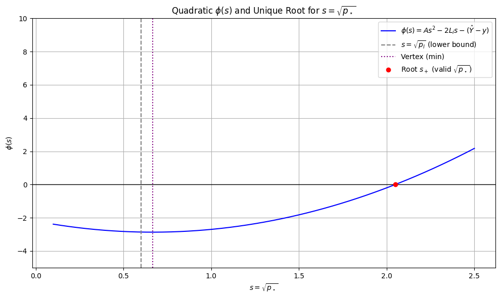
There exists one unique solution that lies in the range $(0, u]$ and that solution is given by: $s_+ = \frac{-L + \sqrt{L^2 + A(\hat Y+y)}}{A}$

Let's take the above quadratic as a function $\phi(s)$ s.t. $\phi(\sqrt{p_\star}) = 0$:

$\phi(s) =A s^2 + 2Ls - (\hat Y+y)$

Lemma 1: Monotonicity of $\phi(s)$ over $(0,u]$

We prove that $\phi(s)$ monotonically increases for $s \in (0, u]$ by showing that $\phi'(s) \ge 0$ in that range:

$\phi'(s) = 2As + 2L$

$\phi'(0) \ge 0$: $\phi'(0) = 2A(0) + 2L = 2L \Rightarrow \phi'(0) \ge 0$

$\phi'(u) \ge 0$:

• Expand $\phi'(u)$: $2Au + 2L \ge 0 \Leftrightarrow 2 (B + \tilde X - x)u \ge -2L$
• Prove tighter bound: $B + \tilde X - x \ge -x \Rightarrow 2(-x)u \ge -2L \Rightarrow 2Au \ge -2L$
• Use $u = \sqrt\frac{y}{x}$: $\quad 2 (-x)\sqrt{\frac{y}{x}}\ge -2\sqrt{xy}\Leftrightarrow x\sqrt{\frac{y}{x}}\le\sqrt{xy}\Leftrightarrow\sqrt{x^2\frac{y}{x}}=\sqrt{xy}$

Lemma 2: Boundary signs $\phi(0) < 0$ and $\phi(u) \ge 0$

$\phi(0) \lt 0$: $- (\tilde Y + y) < 0$ $\phi(u) \ge 0$:

• Expand $\phi(u)$: $Au^2+2Lu-(\tilde Y + y) \ge 0$
• Expand $A$ and simplify: $(B + \hat X - x)u^2+2y-\tilde Y - y \ge 0 \Leftrightarrow (B + \tilde X)u^2 \ge \tilde Y$
• Reorganize & expand $u^2$: $p_{i+1}\ge\frac{\tilde Y}{B + \tilde X}$
• Recognize that $\tilde p = \frac{\tilde Y}{B + \tilde X}$ and that $p_{i+1} \ge \tilde p$ is the precondition for beginning this calculation

Lemma 3: Unique Solution in $(0,u]$

Using Lemma 1 & 2 and the Intermediate value theorem we now know that there is exactly one $s \in (0,u]$ s.t. $\phi(s) = 0$ and therefore only one solution to the quadratic in that range.

Lemma 4: $s_+$ is that solution

$s_+ = \frac{-L + \sqrt{D}}{A}, D:=L^2 + A(\hat Y+y)$ $s_- = \frac{-L - \sqrt{D}}{A}$

$A > 0$: trivially $s_- < 0$, leaving $s_+$ as the only positive solution.

$A < 0$:

When $A < 0$ then $\sqrt D < L$. This leads to both $s_+$ and $s_-$ being positive. However in this case we can show that:

$s_+ < s_-$ $\frac{-L + \sqrt{D}}{A} < \frac{-L - \sqrt{D}}{A}$ $-L + \sqrt{D} > -L - \sqrt{D}$ $\sqrt{D} > - \sqrt{D}$

All together

Together we've shown that there is always a positive solution for $\sqrt {p_\star}$ that lies between $0$ and $\sqrt{p_{i+1}}$ and that it's calculated via the positive solution from the quadratic.

One-for-Zero (price increasing)

For a given tick $i$ that is being swapped through, we have:

$\Delta x = L\left(\frac{1}{\sqrt{p_i}}-\frac{1}{\sqrt{p_\star}}\right),\qquad\Delta y = L\cdot(\sqrt{p_\star}-\sqrt{p_i}),\qquad B = (\hat X+\Delta x) - \frac{\hat Y+\Delta y}{p_\star}.$

Quadratic in $\sqrt{p_\star}$

Clearing denominators, substituting $A := \tilde X + x - B$ and $s := \sqrt{p_\star}$, simplifying yields:

$As^2 - 2Ls - (\tilde Y - y) = 0$

Solutions:

$$\begin{aligned} \sqrt{p_\star} &= \frac{L \pm \sqrt{L^2 + A(\hat Y - y)}}{A} \\ &= \frac{L \pm \sqrt{\hat Y (x + \hat X - B) - y (\hat X - B)}}{x + \hat X - B}. \end{aligned}$$

Lemma 1: Monotonicity in range $[l, +\infty)$ (where $l = \sqrt{p_i}$)

$$\begin{aligned} \phi'(s) &= 2As - 2L \\ \phi'(s) \ge 0 &\Leftrightarrow s \ge \frac{L}{A} \end{aligned}$$

We'll call the point $\frac L A$ at which $\phi(s)$ becomes monotonically increasing $s_0$ it may or may not lie in the range $[l, +\infty)$

Lemma 2: Negative Lower Range Bound $\phi(s_0) \le 0$

$$\begin{aligned} \phi(s_0) &\le 0 \\ A\left(\frac{L}{A}\right)^2 - 2L\left(\frac{L}{A}\right) - (\tilde Y - y) &\le 0 \\ -\frac{L^2}{A} - (\tilde Y - y) &\le 0 \\ -\frac{L^2}{A} &\le \tilde Y - y \\ -L^2 &\le (\tilde Y - y) A \\ -L^2 &\le \tilde Y A - y (\tilde X - B) - yx \\ 0 &\le \tilde Y A - y (\tilde X - B) \\ y (\tilde X - B) &\le \tilde Y A \end{aligned}$$

$\tilde X - B < 0$:

• Reorganize into fractions: $\frac y A \ge \frac {\tilde Y}{\tilde X - B}$
• Trivially true because $y > 0, A > 0, \tilde Y > 0$

$\tilde X - B > 0$

• Reorganize into fractions: $\frac y {x + (\tilde X - B)} \le \frac {\tilde Y}{\tilde X - B}$
• Tighten inequality: $\frac y x \le \frac {\tilde Y}{\tilde X - B}$
• Trivially true as it's the pre-condition to the computation

Lemma 3: Unique solution in $[s_0, +\infty)$

Using the above lemmas together with a intermediate value theorem we now know that there is a unique solution in this range.

Lemma 4: $s_+ \in [s_0, +\infty)$

$$\begin{aligned} D &:= L^2 + A(\hat Y - y) \\ s_+ &= \frac{L + \sqrt{D}}{A} \\ s_- &= \frac{L - \sqrt{D}}{A} \end{aligned}$$

When $\hat Y-y \ge 0$:

• $A(\tilde Y - y) \ge 0 \Rightarrow D \ge L^2 \Rightarrow \sqrt D \ge L$
• Trivially: $s_- < 0$ leaving $s_+$ as the only positive solution.

When $\hat Y-y \lt 0$:

• $\sqrt D \lt L$ following the above reasoning, meaning both $s_+$ and $s_-$ are positive
• However we can trivially see that $s_+ > s_-$
• Because exactly one solution must lie in $[s_0, +\infty)$ it must be $s_+$ because if it were $s_-$ it would lead to a contradiction requiring $s_+ > s_-$ but also $s_+ \notin [s_0, +\infty)$.

Lemma 5: $s_+ \ge l$

$$\begin{aligned} \frac{L + \sqrt{D}}{A} &\ge l \\ L + \sqrt{D} &\ge l (x + \tilde X - B) \\ L + \sqrt{D} &\ge L + l (\tilde X - B) \\ \sqrt{D} &\ge l (\tilde X - B) \end{aligned}$$

When $\tilde X - B < 0$: Inequality true because left side is positive and left side negative.

When $\tilde X -B \ge 0$:

$$\begin{aligned} D &\ge p_i (\tilde X - B)^2 \\ L^2 + A (\tilde Y - y) &\ge p_i (\tilde X - B)^2 \\ L^2 + A \tilde Y - yx - y(\tilde X - B) &\ge p_i (\tilde X - B)^2 \\ A \tilde Y - y(\tilde X - B) &\ge p_i (\tilde X - B)^2 \\ A \tilde Y &\ge p_i (\tilde X - B)^2 + y(\tilde X - B) \\ A \tilde Y &\ge p_i (\tilde X - B)^2 + p_i x(\tilde X - B) \\ A \tilde Y &\ge p_i (\tilde X - B)\big((\tilde X - B) + x\big) \\ \frac{\tilde Y}{\tilde X - B} &\ge p_i \\ \tilde p &\ge p_i \end{aligned}$$

This is the precondition for the calculation which makes our lemma $s_+ \ge l$ true!

Final Proposition

Thanks to lemmas 3-5 we have now proven the required facts to know that $s_+$ gives us the unique $\sqrt{p_\star}$.